The high-performance of optical, electronic and mechanical devices requires a complete, fast and often in-situ characterization of their properties at the nanoscale. We are developing different bimodal AFM configurations with the aim of analyzing and understanding the performance and response of a wide variety of materials and devices operating in either air or liquid environments.
Generally speaking bimodal AFM is based on the simultaneous excitation and detection of two eigenmodes of the microcantilever, commonly the first and the second mod, although other combination of eigenmodes could be used. The observables of first mode are primarily used to generate the topography of the surface while the observables of the second mode in combination with those of the first mode are used to generate maps of other properties such as Young modulus, damping, indentation, peak force or viscous coefficients.
Three main factors singularize bimodal AFM operation: the coupling between excited modes induced by the nonlinear tip-surface force, the doubling of the number of observables to record information on material properties and the lack of feedback restrictions for the additional excited mode. The eigenmodes of a cantilever have different force constants, quality factors and resonant frequencies; consequently they do not offer the same sensitivity to detect material properties.
Depending on the type of feedback applied to a given excited mode (amplitude, frequency or open loops) different bimodal configurations can be obtained.

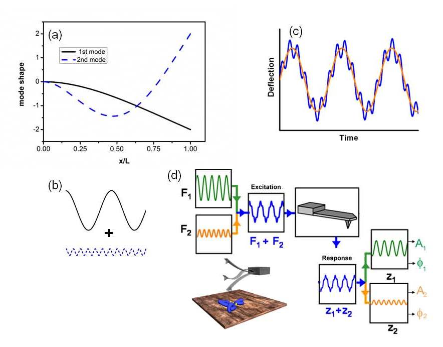
Fig 1. a. Mode shapes of the first two flexural modes of tipless rectangular cantilever beam. b. Scheme of the combination of two frequencies in bimodal AFM and resulting tip excitation c. d. Diagram of bimodal AFM excitation and detection in the AM configuration.

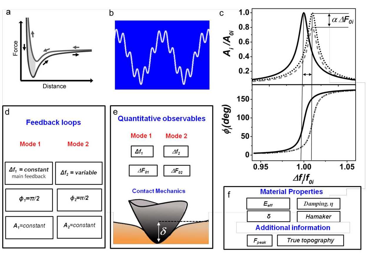
Fig 2. Scheme of bimodal FM-FM. a. Scheme of a force curve. The arrows indicate the direction of the tip motion. b. Tip excitation in bimodal AFM. c. Scheme of the frequency shift, phase shift, amplitude reduction and correction in frequency modulation AFM. d. Block diagram depicting the feedback controls in bimodal nanomechanical spectroscopy. e. Scheme of the main observables and contact mechanics deformation. f. Outcomes of the method.

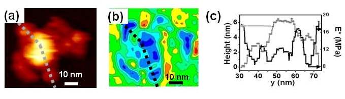
Fig 3. Topography and flexibility mapping of proteins. a) Bimodal AFM topography. b) Flexibility map of a single IgM antibody taken simultaneously with a). c) Flexibility profile along the dashed line marked in b).

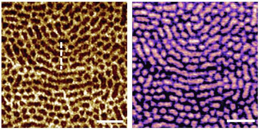
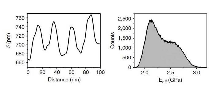
Fig 4. FM bimodal image. These images show the spatial resolution that can be achieved in the nanomechanical maps. a) Indentation map in a block copolymer (PS-b-PMMA) thin film. b) Map of the elastic modulus of PS-b-PMMA. c) Cross-section along the dashed line shown in a). d) Histogram of the elastic modulus obtained from b).

Relevant Publications:
•E.T. Herruzo, A.P. Perrino & R. Garcia. Nat. Commun. 4, 3126 (2014)
•R. Garcia & R. Proksch. Eur. Polym. J. 49, 1897-1906 (2013)
•D. Martinez-Martin, E. T. Herruzo, C. Dietz, J. Gomez-Herrero & R. Garcia, Phys. Rev. Lett. 106, 198101 (2011).
•R. Garcia & E. T. Herruzo, Nature Nanotech.7, 217-226 (2012)
•T.R. Rodriguez and R. Garcia, Appl. Phys. Lett. 84, 3 (2004)